

As known, the US Securities and Exchange Commission (SEC) made a historic decision for the cryptocurrency markets on January 10, approving spot Bitcoin ETF applications. What we are going to do is examine the effect of this decision on the prices after the approval.
To do this, we will use the CausalImpact package from Google. This model uses the structural Bayesian time-series model to understand how the response variable might have evolved after the intervention if the intervention had not occurred. This process is called predicting the counterfactual. In this particular case, the related intervention is the SEC approval.
Now, we will examine Bitcoin prices before and after the approval with the volume (supply size) covariate, that was not affected by the intervention.
library(tidyverse)
library(tidyquant)
library(CausalImpact)
library(zoo)

#Bitcoin USD
df_coin <-
  tq_get("BTC-USD",
         to = "2024-03-17") %>%
  select(date,
         btc = close,
         volume)


#Preparing the response and covariate variables for the zoo object
btc <- df_coin$btc
volume <- df_coin$volume
time_points <-
  seq.Date(as.Date("2014-09-17"),
           by = 1,
           length.out = 3470)

#Building a zoo-data frame
df_zoo <- zoo(cbind(btc, volume),
              time_points)

#pre-intervention period
pre.period <- as.Date(c("2014-09-17", "2024-01-10"))

#post-intervention period
post.period <- as.Date(c("2024-01-11", "2024-03-17"))

#Analyzing the inference
impact <- CausalImpact(df_zoo,
                       pre.period,
                       post.period)

#Plotting causal inference
plot(impact, c("original", "pointwise")) +
  coord_cartesian(xlim = c(as.Date("2023-06-01"),
                           as.Date("2024-03-17"))) +
  scale_x_date(labels = scales::label_date(format = "%Y %b")) +
  theme_bw(base_family = "Bricolage Grotesque")
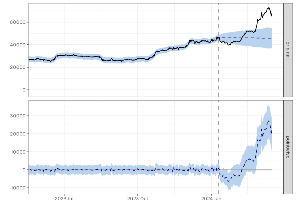
We ignore the cumulative effect because our response variable is a stock quantity (price). So we only show counterfactual (original) and absolute effects (pointwise) on the above plots. The grey dashed line denotes the approval date (intervention). To understand the above charts we better look at the summary statistics.
summary(impact)

#Posterior inference {CausalImpact}

#                         Average          Cumulative
#Actual                   51921            3478717
#Prediction (s.d.)        45956 (2808)     3079032 (188136)
#95% CI                   [40493, 51437]   [2713033, 3446309]

#Absolute effect (s.d.)   6e+03 (2808)     4e+05 (188136)
#95% CI                   [484, 11428]     [32408, 765684]

#Relative effect (s.d.)   13% (7%)         13% (7%)
#95% CI                   [0.94%, 28%]     [0.94%, 28%]

#Posterior tail-area probability p:   0.01131
#Posterior prob. of a causal effect:  98.869%

#For more details, type: summary(impact, "report")
Like I said before, we will ignore the cumulative results. When we look at the averaged relative effect, which stems from 1000 (default) MCMC sampling iterations, we see an approximately 13% increase in the response value. This result is statistically significant because the related interval (95%) does not cover zero.
The p-value of this causal effect is lower than 0.05 (p: 0.01131), which makes the effect statistically significant. Hence, we can say that the approval has an increased effect on the Bitcoin prices.


Leave a comment