

The banking sector has risen since the passing of the orthodox economic policies in Turkey. This article will analyze and model an exchange-traded fund tracking the Turkish banking index for projection for the upcoming year.
library(tidyverse)
library(timetk)

#TCMB(Central Bank of the Republic of Turkey) One-Week Repo Rate
df_tcmb_rates <-
  read_csv("https://raw.githubusercontent.com/mesdi/blog/main/tcmb_funds.csv") %>%
  janitor::clean_names() %>%
  select(date = release_date, tcmb_rates = actual) %>%
  mutate(date = case_when(str_detect(date," \\(.*\\)") ~ str_remove(date," \\(.*\\)"), #removing parentheses and the text within
                          TRUE ~ date) %>%
                parse_date(date, format = "%b %d, %Y") %>%
                floor_date("month") %m+% months(1),
         tcmb_rates = str_remove(tcmb_rates, "%") %>% as.numeric()) %>%
  #makes regular time series by filling the time gaps
  pad_by_time(date, .by = "month") %>%
  tidyr::fill(tcmb_rates, .direction = "up") %>%
  drop_na()

#TAU-BIST Bank Index Equity (TRY) Fund (Equity Intensive Fund)
df_tau <-
  read_csv("https://raw.githubusercontent.com/mesdi/blog/main/tau.csv") %>%
  janitor::clean_names() %>%
  mutate(date = parse_date(date, "%m/%d/%Y")) %>%
  select(date, fund_price = price)

#Merging all the data frames
df_merged <-
  df_tau %>%
  left_join(df_tcmb_rates) %>%
  drop_na()

#Anomaly analysis of the Fund Price
df_merged %>%
  pivot_longer(cols = c(-date), names_to = "vars") %>%
  filter(vars == "fund_price") %>%
  anomalize(date, value) %>%
  plot_anomalies(date)

The anomaly plot of the fund prices confirms that shifting the policies has recently moved the fund values to a sharp upward trend.
We plan to use multiple algorithms to determine the best forecasting method. For this purpose, we will use the tidyAML package to compare all models. However, we will need to add the prophet model externally since it is not included in the package.
#Fast Regression witm many models
library(tidymodels)
library(modeltime)
library(tidyAML)
library(baguette)
library(bonsai)

#Split into a train and test set
splits <-
  df_merged %>%
  timetk::time_series_split(assess = "1 year", cumulative = TRUE)

train <- training(splits)
test <- testing(splits)

#Formula/preprocessing
df_rec <- recipe(fund_price ~ ., data = train)

#Modeling
df_reg <-
  fast_regression(
    .data = df_merged,
    .rec_obj = df_rec,
    .parsnip_fns = c("rand_forest",
                     "bag_tree",
                     "mars",
                     "bag_mars",
                     "boost_tree"
                     ),
    .parsnip_eng = c("ranger",
                     "earth",
                     "rpart",
                     "lightgbm")
  )


#Adding the prophet Model

#Preprocessing/formula
rec_prophet <-
  recipe(fund_price ~ ., data = train)

#Model specification
spec_prophet <-
  prophet_reg() %>%
  set_engine(engine = "prophet")

#Fitting workflow
set.seed(12345)
wflow_fit_prophet <-
  workflow() %>%
  add_recipe(rec_prophet) %>%
  add_model(spec_prophet) %>%
  fit(train)

#Augmented data
prophet_aug <-
  broom::augment(wflow_fit_prophet, new_data = test) %>%
  #Adding engine+function column
  mutate(pfe = "prophet - prophet_reg")


#Plotting residuals distribution of all models
library(ragg)

df_reg %>%
  mutate(res = map(fitted_wflw, \(x) broom::augment(x, new_data = test))) %>%
  unnest(cols = res) %>%
  mutate(pfe = paste0(.parsnip_engine, " - ", .parsnip_fns)) %>%
  select(date,
         fund_price,
         tcmb_rates,
         .pred,
         pfe) %>%
  rbind(prophet_aug) %>%
  mutate(.res = fund_price - .pred) %>%
  ggplot(aes(x = .res,
             y = pfe,
             fill = pfe)) +
  geom_boxplot(show.legend = F) +
  theme_minimal(base_family = "Bricolage Grotesque",
                base_size = 16) +
  labs(title = "Residuals by Fitted Model",
       x = "",
       y = "") +
  theme(plot.title = element_text(hjust = 0.5))
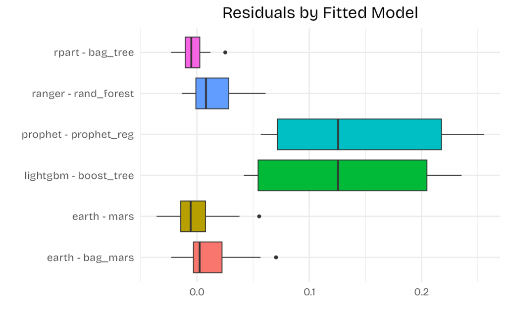
Looking at the above chart, it seems reasonable to eliminate the prophet and lightgbm models from our workflow. We can then recalculate the accuracy of the remaining models and rank them accordingly.
#Modeling with rpart-bag_tree

#Model Specificaiton
mod_rpart <-
  bag_tree() %>%
  set_engine("rpart") %>%
  set_mode("regression")

#Fitting
set.seed(12345)
wflw_fit_rpart <-
  workflow() %>%
  add_recipe(df_rec) %>%
  add_model(mod_rpart) %>%
  fit(train)

#Modeling with ranger-rand_forest

#Model Specificaiton
mod_ranger <-
  rand_forest() %>%
  set_engine("ranger") %>%
  set_mode("regression")

#Fitting
set.seed(12345)
wflw_fit_ranger <-
  workflow() %>%
  add_recipe(df_rec) %>%
  add_model(mod_ranger) %>%
  fit(train)

#Modeling with earth - mars

#Model specification
mod_mars <-
  mars() %>%
  set_engine("earth") %>%
  set_mode("regression")

#Fitting
set.seed(12345)
wflow_fit_mars <-
  workflow() %>%
  add_recipe(df_rec) %>%
  add_model(mod_mars) %>%
  fit(train)

#Modeling with earth-bagged_mars

#Model specification
mod_bagged_mars <-
  bag_mars() %>%
  set_engine("earth") %>%
  set_mode("regression")

#Fitting
set.seed(12345)
wflow_fit_bagged_mars <-
  workflow() %>%
  add_recipe(df_rec) %>%
  add_model(mod_bagged_mars) %>%
  fit(train)

#Adding the fitted models to the model table
models_df <-
  modeltime_table(wflw_fit_rpart,
                  wflw_fit_ranger,
                  wflow_fit_mars,
                  wflow_fit_bagged_mars) %>%
  mutate(.function = c("bag_tree",
                       "rand_forest",
                       "mars",
                       "bag_mars"))


#Calibrating the models
cal_df <- modeltime_calibrate(models_df, new_data = test)

#Accuracy
cal_df %>%
  modeltime_accuracy(metric_set = metric_set(rmse,rsq)) %>%
  arrange(-rsq)

# A tibble: 4 × 6
  .model_id .model_desc .function   .type   rmse   rsq
      <int> <chr>       <chr>       <chr>  <dbl> <dbl>
1         3 EARTH       mars        Test  0.0445 0.885
2         1 RPART       bag_tree    Test  0.106  0.885
3         4 EARTH       bag_mars    Test  0.0510 0.848
4         2 RANGER      rand_forest Test  0.125  0.675
If we take rsq and rmse values into consideration, we’d better pick the mars model for forecasting. We will manually take next year’s tcmb_rates values that reflect predictions based on most economists in Turkey. We will create an additional variable (Price_Index) to see the percentage change from the last price.
#Forecasting

##Future(unseen) data frame
library(tsibble)
library(fable)

date <-
  df_merged %>%
  mutate(date = yearmonth(date)) %>%
  as_tsibble() %>%
  new_data(12) %>%
  as_tibble() %>%
  mutate(date = as.Date(date))

df_future <-
  date %>%
  mutate(tcmb_rates = c(rep(42.5,2),45,rep(50,9)))

#Re-fitting and forecasting

#Calibration data for mars
cal_mars <- modeltime_calibrate(wflow_fit_mars,
                                new_data = df_merged)

#Forecasted data frame
tau_fc <-
  cal_mars %>%
  modeltime_refit(df_merged) %>%
  modeltime_forecast(new_data = df_future) %>%
  select(Date = .index, Fund_Price = .value) %>%
  mutate(Price_Index = (Fund_Price/ first(df_merged$fund_price)*100) %>%
                       round(0), #making 2023 Dec value = 100 to see the changes(%)
         Fund_Price = round(Fund_Price, 3),
         Date = yearmonth(Date))

#Making a forecasting table
library(kableExtra)

tau_fc %>%
  kbl() %>%
  kable_styling(full_width = F,
                position = "center") %>%
  column_spec(column = 3,
              color= "white",
              background = spec_color(tau_fc$Price_Index, end = 0.7)) %>%
  row_spec(0:nrow(tau_fc), align = "c") %>%
  kable_minimal(html_font = "Bricolage Grotesque")

It looks like that will double its value at the end of the coming year.


Leave a comment