

Most of the time, if there is a recession in an economy, it leads to a high unemployment rate, and then it triggers the over-qualified employment rate; Because people would feel financially insecure and they’d accept the first job that comes their way regardless of how the job suit for their skills or education levels.
Over-qualification employment is when people with higher education are employed in jobs that do not require such a high level of education. We will compare over-qualification rates by gender and the women business and the law index. This index measures how laws and regulations affect the opportunities women have in their workforce ecosystems.
First, we create our dataset. Cyprus is assigned to the Western Asia subcontinent in the region23 codelist. This makes it unique in the related subregion. So, I decided to move it to Southern Europe subregion, which is more convenient, in my opinion.
library(tidyverse)
library(rsample)
library(WDI)
library(countrycode)
library(systemfonts)
library(showtext)


df <- read_csv("https://raw.githubusercontent.com/mesdi/blog/main/eu_qlf.csv")

df_qualified <-
  df %>%
  select(-(starts_with("..."))) %>%
  mutate(across(.cols=-(1:2), .fns= ~ str_replace_all(.,":","NA"))) %>%
  mutate(across(.cols = -(1:2), .fns = as.numeric)) %>%
  pivot_longer(-c("country","gender"),
               names_to = "time",
               values_to = "rates") %>%
  mutate(time = as.numeric(time))


#Women Business and the Law Index Score (scale 1-100) - European Union
df_ind <-
  WDI(indicator = "SG.LAW.INDX") %>%
  as_tibble() %>%
  rename(index = SG.LAW.INDX) %>%
  select(-(2:3)) %>%
  na.omit()


df_tidy <-
  df_qualified %>%
  left_join(df_ind,
            by = c("country",
                   "time"="year")) %>%
  mutate(region = countrycode(country,
                              "country.name",
                              "region23")) %>%
  mutate(region = case_when(country == "Cyprus" ~ "Southern Europe",
                            TRUE ~ region),
         axis_color = case_when(region == "Western Europe" ~ "#007300",
                                region == "Eastern Europe" ~ "#e41a1a",
                                region == "Northern Europe" ~ "#9BB7D4",
                                TRUE ~ "#E5E500")) %>%
  na.omit()
Now, we look through how over-qualification rates change by gender and country/region in the EU in a plot.
#Dataset for segment layer
segment_data <-
  df_tidy %>%
  filter(time == 2021) %>%
  pivot_wider(names_from = gender,
              values_from = rates)

#Google font setting
font_add_google("Fira Sans","fira")
showtext_auto()

#Comparing over-qualified rates and index plot
df_tidy %>%
  filter(time == 2021) %>%
  ggplot(aes(x = fct_reorder(country, index),
             y = index)) +
  geom_bar(stat = "unique", # to avoid replicate results
           fill = "navyblue",
           alpha = 0.5) +
  geom_segment(data = segment_data,
               mapping = aes(y = Males,
                             yend = Females,
                             x = country,
                             xend = country),
               color = "orange",
               size =1.2) +
  geom_point(data = segment_data,
             aes(y=Males, x=country),
             color = "#064279",
             size = 3) +
  geom_point(data = segment_data,
             aes(y=Females, x=country),
             color = "#e71892",
             size = 3) +
  #conditional color formatting of the X-axis
  scale_x_discrete(labels = setNames(segment_data$country,
                                     segment_data$axis_color),
                   breaks = segment_data$country) +
  coord_flip() +
  xlab("") +
  ylab("") +
  ggtitle("Comparing Over-qualified Rates of Europe's <span style='color:#007300;'>Western</span>, <span style = 'color:#e41a1a;'>Eastern</span>, <span style = 'color:#9BB7D4;'>Northern</span> and <span style = 'color:#E5E500;'>Southern</span> Regions") +
  labs(subtitle = "by Sex (<span style = 'color:#064279;'>Males</span>-<span style = 'color:#e71892;'>Females</span>) and the <span style='color:#6666b2;'>Women Business and the Law Index Score</span>, 2021") +
  theme_minimal(base_family = "fira",
                base_size = 18) +
  theme(axis.text.y = element_text(colour = segment_data$axis_color),
        plot.title = ggtext::element_markdown(hjust = 0.5, size = 15),
        plot.subtitle = ggtext::element_markdown(hjust = 0.5, size = 15))
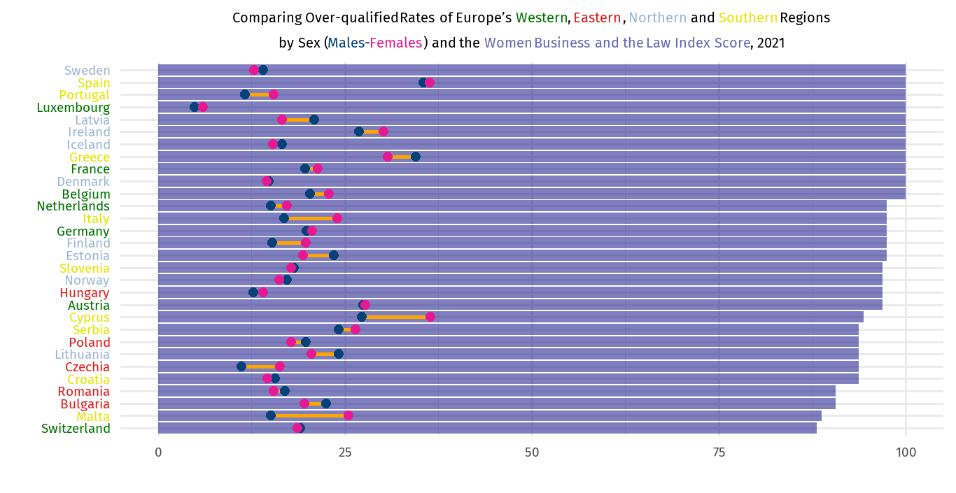
When we look at the above graph, we can see that the Eastern countries have the lowest index scores and highest over-qualification rates. The higher over-qualification rates are predominantly seen in the Southern countries, headed by Spain and Cyprus.
I couldn’t deduce how gender affects the over-qualification rates. To understand the relation, we will bootstrap a linear regression model.
#Bootstrap intervals
set.seed(123)
df_boost <-
  reg_intervals(rates ~ gender + index + region,
                data = df_tidy,
                times = 1e3)


#Explanatory plot by the model coefficients
df_boost %>%
  mutate(term = str_replace(term, "region|gender","")) %>%
  ggplot(aes(.estimate, term)) +
  geom_vline(xintercept = 0,
             size = 1.5,
             lty = 2,
             color = "red") +
  geom_errorbar(size = 1.4,
                alpha = 0.7,
                color = "navyblue",
                aes(xmin = .lower, xmax = .upper)) +
  geom_point(size = 3) +
  xlab("") +
  ylab("") +
  theme_minimal(base_family = "fira",
                base_size = 18)
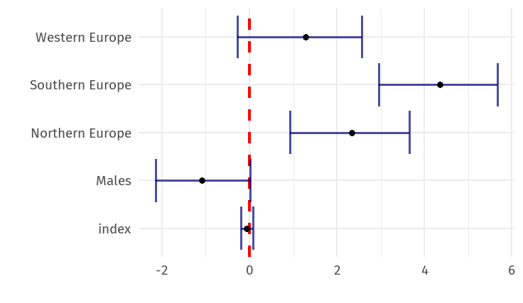
The strange thing about the results is that the index variable does not affect the rates significantly. In addition, it is seen that men have a reduced effect on the rates. So, we might think the opposite is true for women. The results of the sub-regions seem to confirm the first graph.


Leave a comment