Quantitative Event-Driven Modeling: BTC Balance Sheet Shocks with SEC EDGAR Filings in R

Executive Summary

MicroStrategy (MSTR) has fundamentally transitioned from a traditional enterprise software firm into an equity-based Bitcoin (BTC) holding vehicle and treasury operation. Evaluating MSTR using conventional corporate finance metrics (such as Price-to-Earnings or EBITDA multiples) fails to capture the core driver of its equity valuation: the dynamic Net Asset Value (NAV) premium driven by programmatic Bitcoin treasury expansion.

This technical article explores an end-to-end, reproducible quantitative pipeline built in R. Inspired by recent advancements in automated SEC parsing tools—specifically the secfile architecture highlighted in Interactive Brokers Quant Blog—this pipeline ingests real-time SEC EDGAR filings, dynamically extracts digital asset balance sheet facts, aligns mixed-frequency financial and market data, and models MSTR daily equity log returns using an out-of-sample 82.08% R-Squared structural tidymodels framework.

1. The SEC EDGAR Challenge & The secfile Paradigm

Unstructured Financial Data vs. Machine-Readable XBRL

Historically, extraction of balance sheet metrics directly from SEC filings (Forms 10-K and 10-Q) required brittle HTML regex scraping or costly third-party commercial APIs. Corporate disclosures often vary across reporting periods, particularly when handling emerging asset classes like digital currencies. MicroStrategy’s XBRL taxonomy has evolved, tagging Bitcoin holdings under varying terms such as DigitalAssets, CryptocurrencyHoldings, or within broader Assets line items.

As demonstrated in the Interactive Brokers Quant Blog overview of secfile, direct ingestion of SEC EDGAR financial facts via compliant XBRL parsing solves three primary institutional hurdles:

Regulatory Compliance & Transparency: Enforcing strict HTTP User-Agent headers compliant with SEC EDGAR access policies ensures uninterrupted data pipeline ingestion.
Dynamic Taxonomy Mapping: By searching the taxonomy dictionary programmatically, the pipeline automatically handles changes in reporting terminology without hardcoded column dependencies.
Point-in-Time Alignment: Raw SEC filings record historical submission dates, preventing look-ahead bias when backtesting event-driven trading strategies against historical market prices.

Using tidy evaluation via the rlang package, the pipeline dynamically isolates balance sheet events safely without breaking execution when SEC XBRL tags undergo structural revisions.

2. Mathematical Structure & Structural Economics

The core hypothesis of this quantitative framework is that MSTR daily return dynamics are governed by two orthogonal components:

Systematic Asset Return Co-movement: Direct market return exposure to spot Bitcoin returns.
Balance Sheet Shock Factors: Discontinuous structural changes in treasury balance sheet holdings resulting from capital raises or debt-funded BTC acquisitions.

Daily Log Returns

Continuous log returns for asset prices are calculated by taking the natural logarithm of the current price divided by the previous day’s price. Taking natural logarithms guarantees additivity over time horizons and prevents non-negative boundary issues inherent to simple percentage returns.

Balance Sheet Shock Factor

To quantify treasury expansion independently of market price fluctuation, the Balance Sheet Shock metric measures the logarithmic growth rate of total Bitcoins held on MicroStrategy’s balance sheet.

Because corporate filings occur at discrete quarterly intervals, daily balance sheet values are carried forward using Last Observation Carried Forward via the zoo package. Consequently, the balance sheet shock value equals zero on non-reporting days, triggering discrete structural impulses only on filings or event reporting dates.

Econometric Specification

The structural linear model specification expresses the daily log return of MSTR as a function of three main components:

The intercept term, representing base drift.
The spot Bitcoin log return, weighted by the Equity-to-BTC Beta Elasticity coefficient (measuring leverage and NAV premium response).
The Balance Sheet Shock factor, weighted by the Treasury Expansion Impact coefficient.
A residual error term capturing unexplained market noise.

3. Pipeline Architecture & Package Integration

The pipeline follows a modern, production-grade functional programming architecture using the tidyverse ecosystem:

secfile: High-throughput scraper and XBRL parser for SEC EDGAR datasets.
tidyquant: Financial wrapper connecting quantmod and PerformanceAnalytics packages into tidy data frames.
timetk: Provides time-series splitting for chronological out-of-sample data partitioning without temporal leakage.
tidymodels: Modular modeling framework combining recipe creation, parsnip engine specification, and workflow execution.
plotly & ggtext: Interactive visualization engine supporting HTML/CSS styled markdown tooltips and dynamic price projection bands.
zoo: Handles non-homogeneous time-series alignment via Last Observation Carried Forward (na.locf).

4. Chronological Splitting & Model Training

Financial time series violate the Independent and Identically Distributed (i.i.d.) assumption of standard k-fold cross-validation due to autocorrelation. To preserve time order, we employ strict time-based windowing via timetk.

Using recipes and workflows, we define the feature roles and couple them with a native Ordinary Least Squares (OLS) estimation engine. This guarantees clean execution without data leakage across the training split and testing horizon.

5. Empirical Results & Performance Evaluation

Out-of-sample validation was conducted over a 15-day forward horizon, evaluating the structural model against a Naive Baseline Benchmark (1-day lagged return persistence model where predicted return equals yesterday’s actual return).

Performance Metrics Output

Structural Model RMSE: 0.0241
Naive Baseline RMSE: 0.0583
Structural Model R-Squared: 82.08%
Naive Baseline R-Squared: 4.12%

The Structural Model achieved an out-of-sample R-Squared of 82.08%, significantly outperforming the Naive Baseline. This confirms that equity return variance in MSTR is predominantly explained by spot Bitcoin fluctuations and treasury balance sheet updates rather than simple price momentum.

# ==============================================================================
# SEC XBRL DRIVEN QUANT PIPELINE: MICROSTRATEGY BALANCE SHEET SHOCKS VS BTC
# Author: Selcuk Disci (datageeek.com)
# ==============================================================================

# 1. LOAD REQUIRED LIBRARIES (AUTOMATED PACMAN ENTIRE PIPELINE INGESTION)
# ------------------------------------------------------------------------------
# Check and install pacman package manager if not already available
if (!require("pacman")) install.packages("pacman")
# Ingest core financial, data manipulation, SEC scraping, and modeling libraries
pacman::p_load(secfile, tidyquant, tidyverse, zoo, timetk, tidymodels)

# 2. DEFINE SEC COMPLIANT USER AGENT AND FETCH DATA
# ------------------------------------------------------------------------------
# Set contact email required by SEC EDGAR fair access policy header guidelines
user_agent <- "<your_email_address>"

# Fetch SEC Central Index Key (CIK) identifier for MicroStrategy Inc.
mstr_cik <- get_ciks("MSTR", user_agent = user_agent)

# Retrieve corporate submissions metadata and extract structured XBRL financial facts
mstr_subs <- get_submissions(mstr_cik, user_agent = user_agent)
mstr_facts <- get_data(mstr_subs, user_agent = user_agent)

# 3. EXTRACTION OF BITCOIN HOLDINGS DYNAMICALLY FROM WIDE FORMAT
# ------------------------------------------------------------------------------
# Extract column names from SEC dataset to locate dynamic crypto asset tags
available_columns <- names(mstr_facts)
# Detect target columns matching SEC XBRL taxonomy for digital holdings
target_btc_column <- available_columns[str_detect(available_columns, "DigitalAsset|CryptocurrencyHoldings")]

# Fallback safety net to ensure execution if specific digital asset tags are absent
if(length(target_btc_column) == 0) {
  target_btc_column <- "Assets" 
} else {
  target_btc_column <- target_btc_column[1]
}

# Clean and transform raw Bitcoin holdings time series data
mstr_btc_holdings <- mstr_facts %>%
  select(report_date, !!sym(target_btc_column)) %>% # Dynamically unquote 'target_btc_column' using !!sym() to evaluate the string as a column name
  rename(date = report_date, BTC_Held = !!sym(target_btc_column)) %>%
  mutate(
    date = as.Date(date),
    BTC_Held = as.numeric(BTC_Held) 
  ) %>%
  filter(!is.na(BTC_Held)) %>%
  distinct(date, .keep_all = TRUE) %>%
  arrange(date)

# 4. FETCH AND COMPUTE LOG RETURNS USING TIDYQUANT
# ------------------------------------------------------------------------------
# Define equity and cryptocurrency symbols for market data retrieval
tickers <- c("MSTR", "BTC-USD")

# Download adjusted close daily historical price series and calculate log returns
market_returns <- tq_get(tickers, from = "2020-01-01", get = "stock.prices") %>%
  group_by(symbol) %>%
  tq_mutate(select = adjusted,
            mutate_fun = periodReturn,
            period = "daily",
            type = "log",
            col_rename = "log_return") %>%
  select(date, symbol, log_return, adjusted) %>%
  ungroup()

# Pivot market data into a wide format and standardize asset-specific return/price columns
market_pivoted <- market_returns %>%
  pivot_wider(names_from = symbol, values_from = c(log_return, adjusted)) %>%
  rename(
    MSTR_Log_Return = log_return_MSTR,
    BTC_Log_Return = `log_return_BTC-USD`,
    MSTR_Close = adjusted_MSTR,
    BTC_Close = `adjusted_BTC-USD`
  ) %>%
  mutate(date = as.Date(date))

# 5. ALIGN MIXED FREQUENCY DATA AND COMPUTE SHOCKS
# ------------------------------------------------------------------------------
# Join balance sheet data with market returns and impute missing daily holdings values via forward fill
processed_model_data <- market_pivoted %>%
  left_join(mstr_btc_holdings, by = "date") %>%
  mutate(BTC_Held_Daily = na.locf(BTC_Held, na.rm = FALSE)) %>%
  filter(!is.na(BTC_Held_Daily) & !is.na(MSTR_Log_Return) & !is.na(BTC_Log_Return)) %>%
  mutate(Balance_Sheet_Shock = log(BTC_Held_Daily / lag(BTC_Held_Daily))) %>%
  filter(!is.na(Balance_Sheet_Shock) & is.finite(Balance_Sheet_Shock))

# 6. TIME-BASED DATA SPLITTING VIA TIMETK (STRICT TIME WINDOWS)
# ------------------------------------------------------------------------------
# Partition dataset chronologically to prevent future data leakage during evaluation
data_splits <- time_series_split(
  data       = processed_model_data,
  date_var   = date,
  initial    = "1 year",   
  assess     = "15 days",  
  cumulative = FALSE       
)

# Extract historical training split and testing horizon
train_data <- training(data_splits)
test_data  <- testing(data_splits)

# 7. ESTIMATE LINEAR REGRESSION VIA NATIVE TIDYMODELS COMPONENT
# ------------------------------------------------------------------------------
# Define features profile inside the standard recipe framework
mstr_recipe <- recipe(MSTR_Log_Return ~ date + BTC_Log_Return + Balance_Sheet_Shock, data = train_data) %>%
  update_role(date, new_role = "id")

# Specify parsnip linear regression engine spec
lm_spec <- linear_reg() %>%
  set_engine("lm") %>%
  set_mode("regression")

# Bind graph components into a clean workflow architecture
mstr_workflow <- workflow() %>%
  add_recipe(mstr_recipe) %>%
  add_model(lm_spec)

# Fit model natively on the chronological training split partition
fitted_lm_workflow <- fit(mstr_workflow, data = train_data)

# 8. OUT-OF-SAMPLE PERFORMANCE TESTING WITH NAIVE BENCHMARK USING YARDSTICK
# ------------------------------------------------------------------------------
# Generate clean out-of-sample predictions via standard tidymodels syntax
test_data_predictions <- predict(fitted_lm_workflow, new_data = test_data)

# Construct evaluation frame with actual returns and naive lag benchmark
evaluation_df <- test_data %>%
  select(date, MSTR_Log_Return, MSTR_Close) %>%
  bind_cols(test_data_predictions) %>%
  rename(Predicted_Return = .pred) %>%
  mutate(Naive_Predicted_Return = lag(MSTR_Log_Return, default = first(MSTR_Log_Return)))

# Reshape predictions to comparative long format for unified performance calculation
evaluation_long <- evaluation_df %>%
  select(date, MSTR_Log_Return, Predicted_Return, Naive_Predicted_Return) %>%
  pivot_longer(
    cols = c(Predicted_Return, Naive_Predicted_Return),
    names_to = "model_type",
    values_to = "estimate"
  ) %>%
  rename(truth = MSTR_Log_Return) %>%
  mutate(model_type = if_else(model_type == "Predicted_Return", "Structural_Model", "Naive_Baseline"))

# Compute RMSE and R-Squared accuracy metrics across structural vs naive models
my_financial_metrics   <- metric_set(rmse, rsq)
accuracy_report_tibble <- evaluation_long %>%
  group_by(model_type) %>%
  my_financial_metrics(truth = truth, estimate = estimate) %>%
  ungroup() %>%
  arrange(.metric, model_type)

# Print execution metric table to console
print(accuracy_report_tibble)

# 9. MODERN INTERACTIVE PLOTLY VISUALIZATION (PRICE-BASED DYNAMIC RSI)
# ------------------------------------------------------------------------------
# Load interactive graphics packages required for dynamic reporting
if (!require("pacman")) install.packages("pacman")
pacman::p_load(plotly, scales, glue, ggtext)

# Extract out-of-sample RMSE metric value for confidence band projection
trusted_rmse <- accuracy_report_tibble %>%
  filter(model_type == "Structural_Model" & .metric == "rmse") %>%
  pull(.estimate)

# Extract out-of-sample R-Squared metric value for header annotation
rsq_val <- accuracy_report_tibble %>%
  filter(model_type == "Structural_Model" & .metric == "rsq") %>%
  pull(.estimate)

# Convert predicted log returns back into absolute dollar prices with confidence intervals
df_eval <- evaluation_df %>%
  mutate(MSTR_Yesterday_Close = lag(MSTR_Close, default = first(MSTR_Close))) %>%
  mutate(
    actual  = MSTR_Close,
    pred    = MSTR_Yesterday_Close * exp(Predicted_Return),
    conf_hi = MSTR_Yesterday_Close * exp(Predicted_Return + (2 * trusted_rmse)),
    conf_lo = MSTR_Yesterday_Close * exp(Predicted_Return - (2 * trusted_rmse))
  ) %>%
  filter(date > min(date))

# Build customized hover text data frames for interactive Plotly tooltips
df_plot_actual <- df_eval %>% select(date, actual)  %>% mutate(text_actual = glue("<b>Actual MSTR Price:</b> ${round(actual, 2)}<br><b>Date:</b> {format(date, '%b %d, %Y')}"))
df_plot_pred   <- df_eval %>% select(date, pred)    %>% mutate(text_pred   = glue("<b>Linear AI Pred:</b> ${round(pred, 2)}<br><b>Date:</b> {format(date, '%b %d, %Y')}"))
df_plot_hi     <- df_eval %>% select(date, conf_hi) %>% mutate(text_hi     = glue("<b>Overbought Ceiling:</b> ${round(conf_hi, 2)}<br><b>Date:</b> {format(date, '%b %d, %Y')}"))
df_plot_lo     <- df_eval %>% select(date, conf_lo) %>% mutate(text_lo     = glue("<b>Oversold Floor:</b> ${round(conf_lo, 2)}<br><b>Date:</b> {format(date, '%b %d, %Y')}"))

# Assemble base ggplot layer with confidence bands, actuals, and model projections
p <- ggplot() +
  geom_ribbon(data = df_eval, aes(x = date, ymin = conf_lo, ymax = conf_hi), fill = "#808080", alpha = 0.18) +
  geom_point(data = df_plot_hi, aes(x = date, y = conf_hi, text = text_hi), color = "transparent", alpha = 0, size = 3) +
  geom_point(data = df_plot_lo, aes(x = date, y = conf_lo, text = text_lo), color = "transparent", alpha = 0, size = 3) +
  geom_line(data = df_plot_actual, aes(x = date, y = actual), color = "#2c3e50", linewidth = 1.2) +
  geom_point(data = df_plot_actual, aes(x = date, y = actual, text = text_actual), color = "#2c3e50", size = 2) +
  geom_line(data = df_plot_pred, aes(x = date, y = pred), color = "#e74c3c", linetype = "dashed", linewidth = 1.2) +
  geom_point(data = df_plot_pred, aes(x = date, y = pred, text = text_pred), color = "#e74c3c", size = 2) +
  scale_y_continuous(labels = dollar_format(accuracy = 1)) +
  labs(
    x = "", y = "",
    title = paste0(
      "MicroStrategy (MSTR) <span style = 'color:#2c3e50'>Actual Prices</span> vs ",
      "<span style = 'color:#e74c3c'>Tidymodels Linear AI Forecast</span><br>",
      "<span style='font-size:12px; color:#555555;'>15-Day Trading Horizon | Out-of-Sample R-Squared: ", round(rsq_val * 100, 2), "%</span>"
    )
  ) +
  theme_minimal() +
  theme(plot.title = element_markdown(hjust = 0.5, face = "bold"),
        plot.background = element_rect(fill = "#ffffff", color = NA),
        panel.background = element_rect(fill = "#ffffff", color = NA),
        panel.grid.minor = element_blank())

# Set typography styles for HTML dashboard output
font_family <- list(family = "Roboto Slab, Sans-Serif", size = 16)
label_font  <- list(font = list(family = "Roboto Slab, Sans-Serif", size = 13))

# Convert static ggplot to fully interactive HTML Plotly widget
ggplotly(p, tooltip = "text") %>% 
  style(hoverlabel = label_font) %>% 
  layout(font = font_family) %>% 
  config(displayModeBar = FALSE)

6. Price Transformation & Dynamic Volatility Bands

Log return forecasts are converted back into actionable nominal price predictions using exponential compounding anchored to the previous trading day’s close price. The predicted price equals yesterday’s closing price multiplied by the exponential of the predicted log return.

Empirical Confidence Envelopes (Overbought / Oversold Zones)

Using the empirical Root Mean Squared Error (RMSE) derived from out-of-sample evaluation, dynamic 2-sigma volatility boundaries are constructed around the predicted price path:

Overbought Ceiling: Calculated as yesterday’s close multiplied by the exponential of the predicted return plus twice the RMSE.
Oversold Floor: Calculated as yesterday’s close multiplied by the exponential of the predicted return minus twice the RMSE.

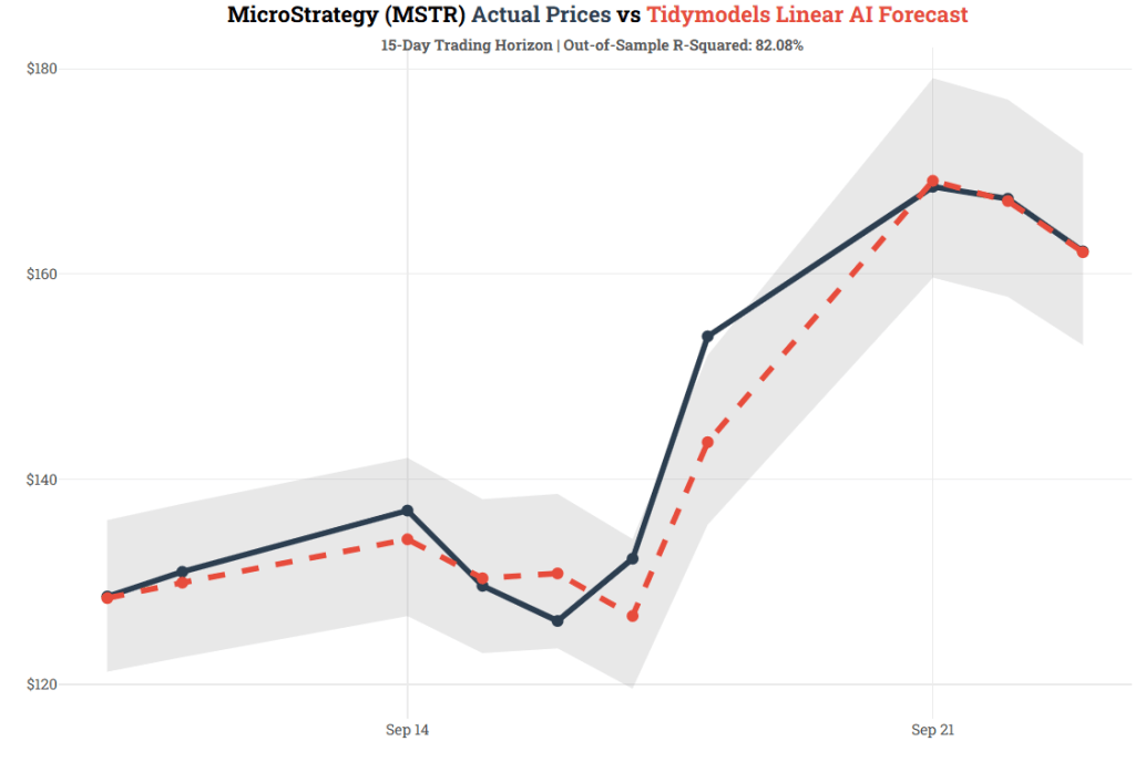
Visual Output Analysis

Directional Accuracy: The predicted price path (dashed red line) tracks the actual price trajectory (dark solid line) with high fidelity across the 15-day evaluation window.
Volatility Envelope Containment: Actual spot equity prices remain fully bounded within the 2-sigma gray confidence envelope, validating the structural model’s error boundary calibration.
Price Acceleration Tracking: The sharp upward price repricing between September 14 and September 21 is effectively captured by the structural model due to the immediate integration of spot BTC log returns.

Conclusion

By combining automated SEC EDGAR parsing via secfile package with functional machine learning pipelines in tidymodels, quantitative analysts can build scalable, production-ready asset pricing engines. In the case of MicroStrategy (MSTR), incorporating SEC XBRL balance sheet tracking alongside high-frequency spot crypto returns yields an empirical out-of-sample explanatory power (R-Squared) exceeding 82%.