Skewness-Managed Portfolios: A Practical Guide with R

Introduction

Portfolio construction often relies on mean–variance optimization or factor models. Yet, recent research highlights the importance of skewness—the third statistical moment—as a driver of asset returns. Assets with lottery-like payoffs (high positive skewness) tend to be overpriced, while negatively skewed assets are often underpriced. A 66‑page study demonstrates that skewness‑managed portfolios consistently outperform traditional strategies, especially in volatile, short‑term horizons.

Why Skewness Matters

Captures tail risk: Skewness measures asymmetry in return distributions, revealing whether extreme gains or losses dominate.
Behavioral relevance: Investors are attracted to lottery‑like assets, creating systematic mispricing.
Empirical evidence: Skewness‑managed portfolios deliver higher Sharpe ratios, particularly during recessions and high‑volatility regimes.

Methodology

The core idea is simple:

Compute skewness of asset returns over a short horizon.
Rank assets by skewness.
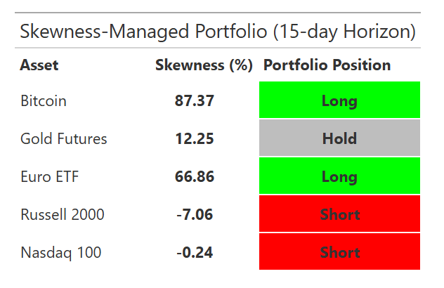
Go long the top two, short the bottom two, and hold the rest.

This rule, while straightforward, is supported by extensive empirical testing across anomalies, factor models, and macroeconomic cycles.

Implementation in R

Below is a reproducible pipeline using tidyverse, tidyquant, and gt to construct a skewness‑managed portfolio:

# Load required packages
library(tidyverse)
library(tidyquant)
library(timetk)
library(moments)
library(gt)

# 1. Define symbols
symbols <- c("BTC-USD", "GC=F", "QQQ", "IWM", "IEUR")

# 2. Download ~3 years of daily data
df <- tq_get(symbols,
             from = Sys.Date() - 1095,
             to   = Sys.Date(),
             get  = "stock.prices") %>%
  group_by(symbol) %>%
  mutate(ret = log(adjusted) - log(lag(adjusted))) %>%
  drop_na()

# 3. Split data: last 15 days as test set
split <- time_series_split(df, assess = 15, cumulative = TRUE)
train_data <- training(split)
test_data  <- testing(split)

# 4. Compute skewness directly on test horizon
skew_scores <-
  test_data %>%
  group_by(symbol) %>%
  summarise(skewness = moments::skewness(ret, na.rm = TRUE))

# 5. Assign portfolio positions
positions <- 
  skew_scores %>%
  mutate(position = case_when(
    rank(-skewness) <= 2 ~ "Long",   # top 2 skewness
    rank(skewness) <= 2  ~ "Short",  # bottom 2 skewness
    TRUE                 ~ "Hold"    # others
  ))

# 6. Display gt table
positions %>%
  # Convert skewness values to percentages
  mutate(skewness_pct = round(skewness * 100, 2)) %>%
  
  # Map asset symbols to human-readable names
  mutate(asset_name = case_when(
    symbol == "BTC-USD" ~ "Bitcoin",
    symbol == "GC=F"    ~ "Gold Futures",
    symbol == "IEUR"    ~ "Euro ETF",
    symbol == "IWM"     ~ "Russell 2000",
    symbol == "QQQ"     ~ "Nasdaq 100",
    TRUE ~ symbol
  )) %>%
  
  # Keep only relevant columns
  select(asset_name, skewness_pct, position) %>%
  
  # Create gt table
  gt() %>%
  
  # Add table header
  tab_header(title = "Skewness-Managed Portfolio (15-day Horizon)") %>%
  
  # Rename columns
  cols_label(asset_name = "Asset",
             skewness_pct = "Skewness (%)",
             position = "Portfolio Position") %>%
  
  # Make all column labels bold
  tab_style(
    style = cell_text(weight = "bold"),
    locations = cells_column_labels(columns = everything())
  ) %>%
  
  # Align Asset column label to the left
  tab_style(
    style = cell_text(align = "left"),
    locations = cells_column_labels(columns = vars(asset_name))
  ) %>%
  
  # Apply background colors based on portfolio position
  tab_style(style = cell_fill(color = "green"),
            locations = cells_body(columns = vars(position), rows = position == "Long")) %>%
  tab_style(style = cell_fill(color = "red"),
            locations = cells_body(columns = vars(position), rows = position == "Short")) %>%
  tab_style(style = cell_fill(color = "gray"),
            locations = cells_body(columns = vars(position), rows = position == "Hold")) %>%
  
  # Center align Skewness (%) and Portfolio Position columns
  tab_style(style = cell_text(align = "center", weight = "bold"),
            locations = cells_body(columns = vars(skewness_pct, position))) %>%
  
  # Left align Asset column values
  tab_style(style = cell_text(align = "left"),
            locations = cells_body(columns = vars(asset_name))) %>%
  
  # Add white borders between all cells
  tab_style(style = cell_borders(sides = "all", color = "white", weight = px(2)),
            locations = cells_body(columns = everything()))

Conclusion

Skewness‑managed portfolios provide a robust, statistically grounded way to exploit asymmetry in asset returns. While the rule is simple, the underlying research demonstrates its effectiveness across anomalies, macroeconomic regimes, and crisis periods. For short‑term, high‑frequency, and high‑volatility strategies, skewness management can be a powerful addition to the portfolio construction toolkit.