Plastic wastes are one of the most dominant pollution factors in the environment as we live in an era where modern industries exist. The most dangerous part of this kind of pollution is mismanaged plastic waste, which ends up mixing into the ocean in the end.
Our World in Data, which we’ll be taking the data for this article, claims that lower-middle countries have the worst waste management systems. Therefore, we will examine the 20 countries that produce the most mismanaged waste based on their GNI income status.
library(tidyverse)
library(tidymodels)
library(janitor)
library(rvest)
library(scales)
library(bbplot)
library(vip)


#Scraping the GNI data set
url <- "https://en.wikipedia.org/wiki/List_of_countries_by_GNI_(nominal)_per_capita"

list_html <-
  read_html(url) %>% #scraping the interested web page
  rvest::html_elements("table.wikitable") %>% # takes the tables we want
  rvest::html_table()


#gni income levels vector
status <- c("high","high","upper_middle","upper_middle",
            "lower_middle","lower_middle","low","low")

#Building and tidying GNI dataframe
df_gni <-
  #assigning the gni income levels to the corresponding countries
  map(1:8,function(x) list_html[[x]] %>% mutate(gni_status=status[x])) %>%
  do.call(what=rbind) %>% #unlisting and merging
  clean_names() %>%#merge gaps with the underscore and makes the capitals lowercase
  mutate(gni_status = as_factor(gni_status)) %>%
  select(country, gni_metric=gni_per_capita_us_1, gni_status) %>%
  mutate(gni_metric = str_remove(gni_metric,",") %>% as.numeric())


#Building and tidying waste dataframe
df_waste <- read_csv("https://raw.githubusercontent.com/mesdi/plastic-pollution/main/plastic-waste-mismanaged.csv")


df_waste <-
  df_waste %>%
  clean_names() %>%
  na.omit() %>%
  select(country=entity,
         waste_metric= mismanaged_plastic_waste_metric_tons_year_1)#renaming


#Binding waste and gni dataframes by country
df_tidy <-
  df_waste %>%
  left_join(df_gni) %>%
  distinct(country, .keep_all = TRUE) %>% #removes duplicated countries
  filter(!country=="World") %>%
  na.omit()

#Top 6 countries in terms of the amounts of mismanaged plastic waste
#to put their amount on the graph
df_6 <-
  df_tidy %>%
  slice_max(order_by=waste_metric, n=6) %>%
  mutate(waste= paste0(round(waste_metric/10^6,2)," million t"))
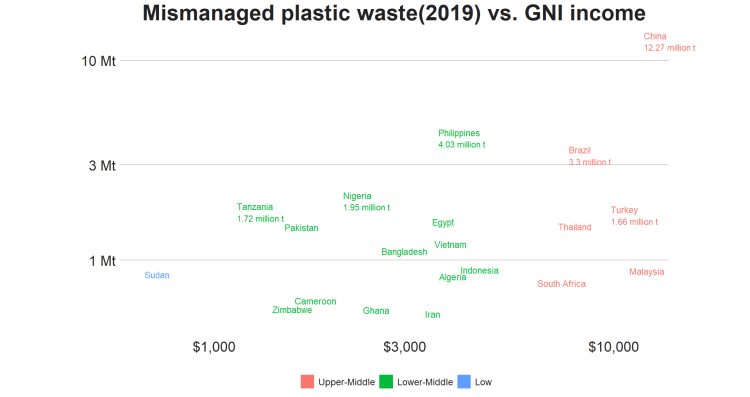
We can now plot the mismanaged plastic waste versus GNI per capita.
#The chart of the top 20 countries in terms of the amounts of plastic wastes
#versus GNI income status
df_tidy %>%
  slice_max(order_by= waste_metric, n=20) %>%
  ggplot(aes(x= gni_metric, y= waste_metric, color= gni_status))+
  geom_text(aes(label= country),
            hjust= 0,
            vjust= -0.5,
            size=4,
            #legend key type
            key_glyph= "rect")+
  geom_text(data = df_6,
            aes(x=gni_metric, y= waste_metric,label=waste),
            hjust=0,
            vjust=1.2)+
  #Using scale_*_log10 to zoom in data on the plot
  scale_x_log10(labels = scales::label_dollar(accuracy = 2))+
  scale_y_log10(labels = scales::label_number(scale_cut = cut_si("t")))+
  scale_color_discrete(labels = c("Upper-Middle","Lower-Middle","Low"))+
  labs(title= "Mismanaged plastic waste(2019) vs. GNI income")+
  coord_fixed(ratio = 0.5, clip = "off")+#fits the text labels to the panel
  bbc_style()+
  theme(
    legend.position = "bottom",
    legend.text = element_text(size=12),
    plot.title = element_text(hjust=0.5)#centers the plot title
  )

When we examine the above graph, we can see that there are no high-income countries in the top 20. China leads by far on the list. The top six countries’ amounts have been written on the corresponding labels.
#Modeling with tidymodels

#preprocessing
df_rec <-
  recipe(waste_metric ~ gni_status, data = df_tidy) %>%
  step_log(waste_metric, base = 10) %>% #stabilizing the variance
  step_dummy(gni_status)

#modeling
lm_model <-
  linear_reg() %>%
  set_engine("lm")

#workflow set
lm_wflow <-
  workflow() %>%
  add_model(lm_model) %>%
  add_recipe(df_rec)


lm_fit <- fit(lm_wflow, df_tidy)

#Descriptive and inferential statistics
lm_fit %>%
  extract_fit_engine() %>%
  summary()


#Call:
#stats::lm(formula = ..y ~ ., data = data)

#Residuals:
#    Min      1Q  Median      3Q     Max
#-3.2425 -0.6261  0.1440  0.8061  2.6911

#Coefficients:
#                        Estimate Std. Error t value
#(Intercept)               3.5666     0.1583  22.530
#gni_status_upper_middle   0.8313     0.2375   3.501
#gni_status_lower_middle   1.5452     0.2409   6.414
#gni_status_low            1.0701     0.3485   3.071
#                        Pr(>|t|)
#(Intercept)              < 2e-16 ***
#gni_status_upper_middle 0.000627 ***
#gni_status_lower_middle 2.13e-09 ***
#gni_status_low          0.002577 **
#---
#Signif. codes:
#0 ‘***’ 0.001 ‘**’ 0.01 ‘*’ 0.05 ‘.’ 0.1 ‘ ’ 1

#Residual standard error: 1.119 on 137 degrees of freedom
#Multiple R-squared:  0.2384,	Adjusted R-squared:  0.2218
#F-statistic:  14.3 on 3 and 137 DF,  p-value: 3.694e-08
To the results seen above, the model is statistically significant in terms of the p-value(3.694e-08 < 0.05). Also, all the coefficients as well are statistically significant by their p-values. When we look at the R-squared of the model we can say that the model can explain %23 of the change in the target variable.
Finally, we will check the beginning claim that which GNI income status has the most effect on how the relative countries handle plastic waste. We will employ a model-based approach with the vip package.
#model-based variable importance
lm_fit %>%
  extract_fit_parsnip() %>%
  vip(aesthetics = list(color = "lightblue", fill = "lightblue")) +
  theme_minimal()

It is seen that according to the above graph, the lower-middle class is the most determinant factor by far to the other categories in terms of mismanaged plastic waste.


Leave a comment