Introduction

Differential Machine Learning (DML), as introduced in the recent arXiv paper (Differential Machine Learning for 0DTE Options with Stochastic Volatility and Jumps), extends supervised learning by incorporating not only function values but also their derivatives. In financial contexts, this often means sensitivities such as Greeks. However, when direct derivatives are unavailable, we can approximate market dynamics using volatility indicators.

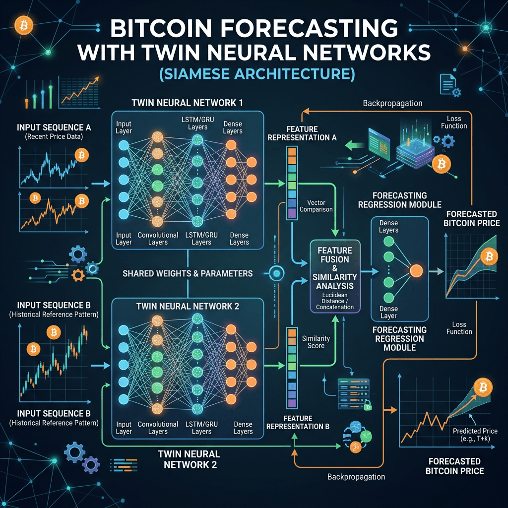
In this project, we adapt DML to Bitcoin price forecasting. Instead of derivatives, we use RSI, MACD, and Bollinger Bands as proxies for volatility. These indicators capture momentum, trend strength, and price dispersion, providing a practical way to embed uncertainty into the learning process. To implement this, we design a twin-network architecture in Keras: one network learns price dynamics from time-based features, while the other learns volatility signals. Finally, we combine them via a stacking ensemble to achieve robust forecasts with confidence intervals.

Why Volatility Variables Instead of Derivatives?

• RSI (Relative Strength Index): Measures momentum and overbought/oversold conditions.
• MACD (Moving Average Convergence Divergence): Captures trend direction and strength.
• Bollinger Bands (upper/lower bands, %B): Quantifies price dispersion and volatility.

These indicators act as empirical substitutes for theoretical derivatives. While DML in its pure form requires sensitivities, in practice, these volatility proxies provide similar information about how prices respond to market forces.

Why Twin Networks?

The idea is to separate the learning tasks:

• The primary network models the continuous component of the price process.
• The auxiliary network models the volatility/jump component. Together, they mimic the decomposition found in stochastic models such as Bates or Heston, but implemented within a flexible neural framework.

Ensemble via Stacking

Once both networks are trained, their predictions are combined using a linear regression meta-model. This stacking ensemble learns the optimal weighting between the primary and auxiliary outputs. The result is a forecast that integrates both trend and volatility signals, significantly improving accuracy compared to either network alone.

Evaluation

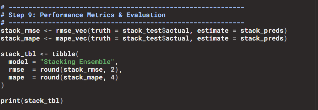
• Metrics: RMSE and MAPE, computed with the yardstick package.
• Results:
  • Individual networks → RMSE ~76,000, MAPE ~99%.
  • Stacking ensemble → RMSE ~3,030, MAPE ~3.65.

This demonstrates the power of combining price and volatility signals in a unified framework.

Confidence Intervals

To quantify uncertainty, we compute residual-based confidence intervals around the point forecasts:

$${\widehat{y}}_t\pm 1.96\cdot {\sigma }_{\text{residuals}}$$

This approach uses the standard deviation of training residuals to generate 95% confidence bands. It provides interpretable uncertainty estimates without requiring explicit probabilistic modeling.

Visualization

The forecasts are visualized with ggplot2:

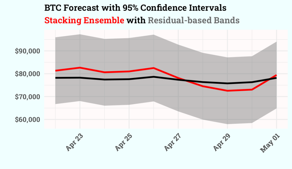
• Grey ribbon → confidence intervals.
• Red line → stacking ensemble forecast.
• Black line → actual BTC prices.

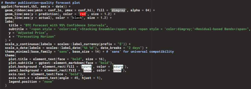
This design clearly communicates both the central forecast and the uncertainty range. The chart you will include at the end of the blog shows exactly this: a red forecast line, black actuals, and a grey confidence band, illustrating how the ensemble integrates volatility information into predictive intervals.

Keras3 in R: Flexible Deep Learning for Financial Forecasting

What is Keras3?

Keras3 is the modern R interface to the Keras deep learning library, built on top of TensorFlow. It allows R users to define, train, and evaluate neural networks with concise syntax while leveraging TensorFlow’s computational power. Unlike earlier versions, Keras3 is fully aligned with TensorFlow 2.x, ensuring long-term support and compatibility.

How We Used Keras3

In our workflow, Keras3 was the backbone for implementing the twin-network architecture:

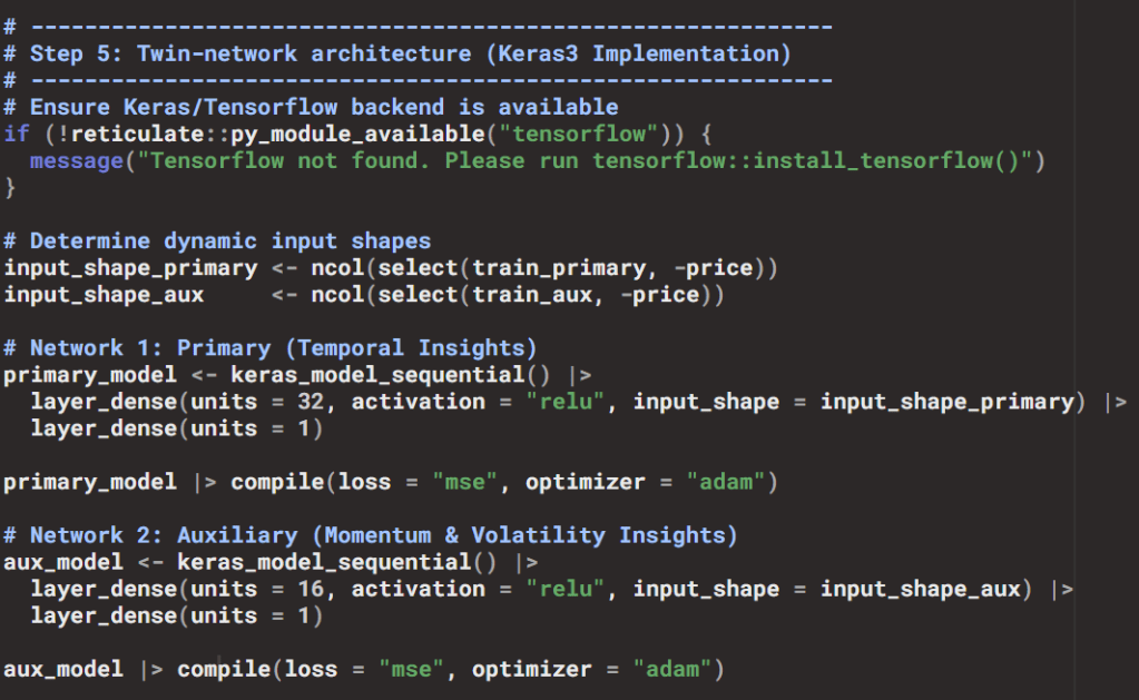
Why ReLU?

• ReLU (Rectified Linear Unit) is the activation function used in hidden layers.
• Formula: $\text{ReLU}(x)=\max (0,x)$.
• Benefits:
  • Introduces non-linearity, enabling the network to learn complex relationships.
  • Efficient and helps avoid vanishing gradients.
  • Well-suited for financial data where signals can be sparse and directional.

Why Adam?

• Adam (Adaptive Moment Estimation) is the optimizer chosen.
• Combines momentum (using past gradients to accelerate learning) and adaptive learning rates (adjusting step sizes per parameter).
• Benefits:
  • Robust for noisy, non-stationary data like cryptocurrency prices.
  • Requires minimal tuning, making it ideal for plug-and-play workflows.
  • Widely adopted in both academic and applied machine learning.

Contribution to the R Ecosystem

Keras3 bridges the gap between R’s tidyverse/tidymodels ecosystem and modern deep learning:

• Integrates seamlessly with data preprocessing pipelines (recipes, timetk).
• Allows financial analysts and data scientists to stay within R while accessing TensorFlow’s deep learning capabilities.
• Encourages reproducibility: models can be defined, trained, and evaluated entirely in R, without switching to Python.
• Expands R’s role beyond traditional statistical modeling into state-of-the-art AI applications.

Why It Matters for DML

By using Keras3:

• We could separate learning tasks into a primary network (trend/seasonality) and an auxiliary network (volatility/momentum).
• Both networks were trained with ReLU activations and Adam optimization, ensuring stability and efficiency.
• Their outputs were combined in a stacking ensemble, yielding forecasts that integrate both price dynamics and volatility signals.

This demonstrates how Keras3 empowers R users to implement advanced architectures like twin networks, making Differential Machine Learning concepts practical in financial forecasting.

Conclusion

This case study demonstrates how Differential Machine Learning concepts can be adapted for financial forecasting in R:

• Volatility indicators serve as practical substitutes for derivatives.
• Twin-network architecture in Keras captures both trend and volatility.
• Stacking ensembles significantly improves predictive performance.
• Residual-based confidence intervals provide interpretable uncertainty estimates.

By combining academic ideas with reproducible R workflows, we can build robust forecasting pipelines that bridge theory and practice.