

Recent advances in time series modeling have emphasized the importance of structural breaks—abrupt changes in the underlying dynamics of financial or economic data. The paper “Directional-Shift Dirichlet ARMA Models for Compositional Time Series with Structural Break Intervention” (Katz, 2026) introduces a Bayesian framework that captures these breaks using three interpretable parameters:
Direction → which component of the composition increases or decreases after a break.
Magnitude (Amplitude) → how large the change is.
Timing → when the break occurs and how quickly the transition unfolds.
This approach ensures that forecasts remain coherent under compositional constraints, while allowing smooth transitions rather than abrupt jumps. In practice, such models are particularly useful when external shocks—like policy changes or crises—reshape the distribution of financial indicators.
Our Bitcoin Volatility Agent
In our collaborative workflow, we implemented a streamlined version of this philosophy for Bitcoin price and volatility analysis:
- Data Wrangling (
tidyverse): Usingdplyrand related tools, we cleaned and transformed the dataset—renaming columns, computing returns, and preparing the series for further analysis. - Volatility Estimation (
zoo): With rolling windows (rollapply), we calculated short‑term volatility measures. This step captures local fluctuations and highlights periods of instability. - Compositional Thinking (
compositions,DirichletReg): Inspired by the paper Directional‑Shift Dirichlet ARMA Models for Compositional Time Series with Structural Break Intervention, we treated volatility regimes as compositional states. While Bitcoin price and volatility are not strictly compositional shares, the Dirichlet regression helps us interpret regime shifts as changes in the balance of market risk over time. - Structural Break Detection (
strucchange): We applied breakpoint analysis to identify regime changes in volatility. This mirrors the paper’s intervention logic—detecting when the underlying dynamics shift due to external shocks. - Bayesian Regression (
MCMCpack): Once regimes were identified, we modeled the Bitcoin price as a function of these regimes. Bayesian inference ensures probabilistic estimates of regime effects, echoing the paper’s emphasis on interpretable parameters (direction, magnitude, timing).
This pipeline mirrors the structural break intervention logic described in Katz’s paper: while the paper formalizes breaks in compositional time series via Dirichlet ARMA dynamics, our agent applies a similar principle to Bitcoin—detecting volatility regimes and quantifying their impact on price.
# Import the core rpy2 interface to communicate with R from Python
import rpy2.robjects as robjects

# Import the package manager interface from rpy2
# This allows us to load and use R packages directly within Python
from rpy2.robjects.packages import importr

# 1. Initialize R's internal package manager
# 'utils' provides functions like install.packages() in R.
utils = importr('utils')

# 2. Define the packages required for the workflow
# These match the R code you executed: data retrieval, wrangling,
# compositional analysis, structural break detection, Bayesian regression, and visualization.
packages = (
    'tidyquant',     # Financial data retrieval (e.g., Bitcoin prices)
    'tidyverse',     # Data wrangling and transformation
    'compositions',  # Compositional data transformations
    'DirichletReg',  # Dirichlet regression models
    'strucchange',   # Structural break detection
    'MCMCpack',      # Bayesian regression and MCMC methods
    'zoo',           # Rolling window functions for volatility
    'ggplot2'        # Visualization
)

print("Checking R packages...")
for p in packages:
    # Check if the package is already installed in R
    check_cmd = f'"{p}" %in% rownames(installed.packages())'
    is_installed_vector = robjects.r(check_cmd)

    # Convert R logical vector to Python boolean
    if is_installed_vector is not None and bool(is_installed_vector[0]):
        print(f"Package '{p}' is already available.")
    else:
        # If not installed, install from CRAN
        print(f"Installing {p} in R. This might take a minute...")
        utils.install_packages(p, repos="https://cloud.r-project.org")

print("\nEnvironment Ready. You can now run your Azure AI Agent code.")
# Import Python's built-in library for interacting with the operating system
import os

# Import httpx, a modern HTTP client for Python
# Used here to handle network requests to Azure OpenAI
import httpx

# Import the Azure OpenAI client
# This allows Python to communicate with Azure-hosted OpenAI models
from openai import AzureOpenAI

# Import the core rpy2 interface to communicate with R from Python
import rpy2.robjects as robjects

# Import pandas2ri for seamless conversion between pandas DataFrames and R data frames
from rpy2.robjects import pandas2ri

# Import localconverter to manage conversion rules between Python and R objects
from rpy2.robjects.conversion import localconverter

# Import display utilities from IPython
# Used to show images (e.g., plots generated by R and saved as PNG files) directly in notebooks
from IPython.display import Image, display

# Connect to Azure OpenAI service
# Configure the client with API version, endpoint, and your API key.
# httpx.Client is used here with SSL verification disabled for simplicity.
client = AzureOpenAI(
    api_version="2025-01-01-preview",
    azure_endpoint="YOUR_URL_ENDPOINT",
    api_key="YOUR_API_KEY",  # replace with your actual key
    http_client=httpx.Client(verify=False, trust_env=False)
)

def run_btc_agent(user_request):
    # Define system instructions for the agent.
    # These instructions enforce raw R code output only.
    # The agent is guided to fetch Bitcoin data, calculate volatility,
    # detect regime shifts, run Bayesian regression, and visualize results.
    system_instructions = (
    "You are a Financial Modeling Agent. Output must be raw R code only, with no explanations, "
    "and never use markdown fences, language tags, or commentary. "
    "Your task is to fetch Bitcoin prices for the last 3 years, calculate volatility, detect regime shifts, "
    "and run Bayesian regression using MCMCpack. Follow these rules:\n"
    "1. Load libraries: tidyquant, tidyverse, compositions, DirichletReg, strucchange, MCMCpack, zoo, ggplot2.\n"
    "2. Fetch Bitcoin data with tq_get('BTC-USD', from = Sys.Date() - years(3), to = Sys.Date()).\n"
    "3. Preprocess: select date and close, rename close -> price, compute returns, "
    "calculate volatility with rollapply(sd), multiply by 100 to express as percentage, drop NA values.\n"
    "4. Regime analysis: use breakpoints(volatility ~ 1, data = btc_data), assign regimes with breakfactor().\n"
    "5. Bayesian regression: run MCMCregress(price ~ regime, data = btc_data) only if regime has at least 2 levels.\n"
    "6. Visualization: create a dual-axis plot with ggplot2. "
    "   • Left y-axis: price (blue line, currency format with dollar sign).\n"
    "   • Right y-axis: volatility (red line, percentage format).\n"
    "   • Rescale volatility for plotting: use btc_data$volatility explicitly in max() calls to avoid closure errors.\n"
    "   • Example: geom_line(aes(y = volatility * max(btc_data$price)/max(btc_data$volatility, na.rm=TRUE))).\n"
    "   • Use scale_y_continuous(name='Price (USD)', labels=scales::dollar_format(), "
    "sec.axis = sec_axis(~ . * max(btc_data$volatility, na.rm=TRUE)/max(btc_data$price), name='Volatility (%)')).\n"
    "   • Lines must be thicker and visually clear.\n"
    "   • Axis text and labels must be bold and bigger, Roboto Slab font.\n"
    "   • Axis titles must be color-coded: blue for Price, red for Volatility. "
    "     Use theme(axis.title.y = element_text(color='blue', face='bold'), "
    "axis.title.y.right = element_text(color='red', face='bold')).\n"
    "   • Title: 'Bitcoin Price & Volatility Analysis'.\n"
    "   • Remove x axis title.\n"
    "   • Remove legend with theme(legend.position = 'none').\n"
    "7. Export: save plot with ggsave('btc_model_plot.png', width=10, height=6, dpi=300)"
)

    # Send the request to Azure OpenAI with system + user instructions
    response = client.chat.completions.create(
        model="gpt-4o",  # name of your deployed model in Azure
        messages=[
            {"role": "system", "content": system_instructions},
            {"role": "user", "content": user_request}
        ]
    )

    # Extract the agent’s R code output
    agent_code = response.choices[0].message.content.strip()
    if agent_code.startswith("```"):
        agent_code = "\n".join(agent_code.split("\n")[1:-1])

    print("-" * 40)
    print(agent_code)
    print("-" * 40)

    try:
        # Execute the R code if it looks valid
        if "library(" in agent_code or "<-" in agent_code:
            with localconverter(robjects.default_converter + pandas2ri.converter):
                cwd = os.getcwd().replace("\\", "/")
                robjects.r(f'setwd(\"{cwd}\")')
                robjects.r(agent_code.strip())

                # Display the generated plot if it exists
                if os.path.exists("btc_model_plot.png"):
                    display(Image(filename="btc_model_plot.png"))
        else:
            print("Skipping execution: output does not look like valid R code.")
    except Exception as e:
        print(f"Agent Error: {e}")

# Run the agent with a specific request
run_btc_agent("Model Bitcoin prices for the last 3 years and provide a volatility analysis.")
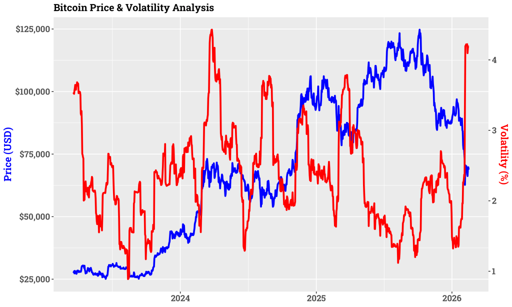
Chart Analysis: Bitcoin Price vs. Volatility (2023–2026)
The dual y-axis chart we generated provides a clear visual of Bitcoin’s dynamics:
Price (blue line): Bitcoin experienced sharp fluctuations, peaking above $100,000 in 2025 before declining in 2026.
Volatility (red line): Volatility rose during periods of rapid price movement, particularly around the 2025 peak, and eased as the market stabilized.
Regime Shifts: The volatility curve suggests distinct phases—low volatility during gradual price increases, followed by heightened volatility during sharp corrections. These regimes align with the structural break analysis, confirming that Bitcoin’s risk profile changes abruptly under market shocks.
Conclusion
By integrating structural break detection with Bayesian regression, our Bitcoin volatility agent offers a practical lens on cryptocurrency risk. The chart illustrates how volatility regimes emerge alongside price swings, echoing the methodological advances in compositional time series modeling.
In short, the agent transforms abstract theory into actionable insight: Bitcoin’s volatility is regime-dependent, and understanding these breaks is key to navigating its unpredictable market.


Leave a comment