

We will try to decide on a fund that is based on the agriculture and food sector indexes for investing. The majority of the fund is based on the Indxx Global Agriculture Net Total Return USD Index. We will take First Trust Indxx Global Agriculture ETF (FTAG) as a reference for this because it fully replicates the index. The other part that makes up around 20-30% is related to the BIST Food Beverage (XGIDA) index.
First, we will model with three different time series forecasting methods:
And we will compare them to find the best model suited to the related time series. When we do that, we will use the bootstrapping and bagging method.
library(tidyquant)
library(timetk)
library(tidyverse)
library(fpp3)
library(seasonal)
library(fable.prophet)
library(tsibble)
library(kableExtra)
library(ragg)
library(plotly)


#BIST Food Beverage (XGIDA)
df_XGIDA <- read_csv("https://raw.githubusercontent.com/mesdi/blog/main/bist_food.csv")

df_xgida <-
  df_XGIDA %>%
  janitor::clean_names() %>%
  mutate(date = parse_date(date,"%m/%d/%Y")) %>%
  select(date, "xgida" = price) %>%
  slice(-1)

#Converting df_xgida to tsibble
df_xgida_tsbl <-
  df_xgida %>%
  mutate(date = yearmonth(date)) %>%
  as_tsibble()

#First Trust Indxx Global Agriculture ETF (FTAG)
df_ftag <-
  tq_get("FTAG", from = "2000-01-01") %>%
  tq_transmute(select = close, mutate_fun = to.monthly) %>%
  mutate(date = as.Date(date)) %>%
  rename("ftag" = close)

#Converting df_ftag to tsibble
df_ftag_tsbl <-
  df_ftag %>%
  mutate(date = yearmonth(date)) %>%
  as_tsibble()


#Merging all the data
df_merged <-
  df_ftag %>%
  left_join(df_xgida) %>%
  drop_na()


#The function of the table of accuracy ranking  of the bagged models
fn_acc <- function(var){
  #Decomposition for bootstrapping preprocess
  stl_train <-
    df_train %>%
    model(STL({{var}}))

  set.seed(12345)
  sim <-
    stl_train %>%
    fabletools::generate(new_data=df_train,
                         times=100,
                         bootstrap_block_size=24) %>%
    select(-.model)

  fit<-
    sim %>%
    model(
      ETS = ETS(.sim),

      Prophet = prophet(.sim ~ season(period = 12,
                                      order = 2,
                                      type = "multiplicative")),

      ARIMA = ARIMA(log(.sim), stepwise = FALSE, greedy = FALSE)
    )

  #Bagging
  fc <-
    fit %>%
    forecast(h = 12)

  #Bagged forecasts
  bagged <-
    fc %>%
    group_by(.model) %>%
    summarise(bagged_mean = mean(.mean))

  #Accuracy of bagging models
  bagged %>%
    pivot_wider(names_from = ".model",
                values_from = "bagged_mean") %>%
    mutate(ARIMA_cor = cor(ARIMA, df_test %>% pull({{var}})),
           ETS_cor = cor(ETS, df_test %>% pull({{var}})),
           Prophet_cor = cor(Prophet, df_test %>% pull({{var}})),
           ARIMA_rmse = Metrics::rmse(df_test %>% pull({{var}}),ARIMA),
           ETS_rmse = Metrics::rmse(df_test %>% pull({{var}}),ETS),
           Prophet_rmse = Metrics::rmse(df_test %>% pull({{var}}),Prophet)) %>%
    as_tibble() %>%
    pivot_longer(cols= c(5:10),
                 names_to = "Models",
                 values_to = "Accuracy") %>%
    separate(Models, into = c("Model","Method")) %>%
    pivot_wider(names_from = Method,
                values_from = Accuracy) %>%
    mutate(cor = round(cor, 3),
           rmse = round(rmse, 2)) %>%
    select(Model, Accuracy = cor, RMSE = rmse) %>%
    unique() %>%
    arrange(desc(Accuracy)) %>%
    kbl() %>%
    kable_styling(full_width = F,
                  position = "center") %>%
    column_spec(column = 2:3,
                color= "white",
                background = spec_color(1:3, end = 0.7)) %>%
    row_spec(0:3, align = "c") %>%
    kable_minimal(html_font = "Bricolage Grotesque")

}


#Modeling the FTAG data

#Splitting the data
df_train <-
  df_ftag_tsbl %>%
  filter_index(. ~ "2022 Sep")

df_test <-
  df_ftag_tsbl %>%
  filter_index("2022 Oct" ~ "2023 Sep")

ftag_table <- fn_acc(ftag)

ftag_table

Now that we have chosen our model for FTAG data, we can use it to make forecasts.
#Bootstraping function
fn_boot <- function(df, var){
  stl_model <-
    {{df}} %>%
    model(STL({{var}}))

  set.seed(12345)
  sim <-
    stl_model %>%
    fabletools::generate(new_data={{df}},
                         times=100,
                         bootstrap_block_size=24) %>%
    select(-.model)
}

#Bagging
sim_ftag <- fn_boot(df_ftag_tsbl, ftag)

fc_ftag<-
  sim_ftag %>%
  model(ETS(.sim)) %>%
  forecast(h = 12)

bagged_ftag <-
  fc_ftag %>%
  summarise(bagged_mean = mean(.mean))
The same process goes for XGIDA data.
#Modeling the XGIDA data

#Splitting the XGIDA data
df_train <-
  df_xgida_tsbl %>%
  filter_index(. ~ "2022 Sep")

df_test <-
  df_xgida_tsbl %>%
  filter_index("2022 Oct" ~ .)

xgida_table <- fn_acc(xgida)

xgida_table

#Bagging
sim_xgida <- fn_boot(df_xgida_tsbl, xgida)

fc_xgida<-
  sim_xgida %>%
  model(ARIMA(log(.sim),
              greedy = FALSE,
              stepwise = FALSE)) %>%
  forecast(h = 12)

bagged_xgida <-
  fc_xgida %>%
  summarise(bagged_mean = mean(.mean))
Finally, we will make a plot to compare the variables and their forecast distributions on the same grid.
#Plot all the series and forecasts in a single chart
ggplot(df_merged, aes(x = date)) +
  geom_line(aes(y = xgida,
                color = "red",
                group = 1,
                text = glue::glue("{yearmonth(date)}\n{round(xgida, 2)}\nXGIDA")),
            size = 1) +
  geom_line(aes(y = ftag*100,
                color = "blue",
                group = 1,
                text = glue::glue("{yearmonth(date)}\n{round(ftag, 2)}\nFTAG")),
            size = 1) +
  geom_line(data = bagged_ftag,
            aes(as.Date(date),
                bagged_mean*100,
                group = "bagged_ftag",
                text = glue::glue("{date}\n{round(bagged_mean, 2)}\nFC_FTAG")),
            size = 1,
            color = "orange",
            linetype = "dotted"
            ) +
  geom_line(data = bagged_xgida,
            aes(as.Date(date),
                bagged_mean,
                group = 1,
                text = glue::glue("{date}\n{round(bagged_mean, 2)}\nFC_XGIDA")),
            size = 1,
            color = "lightblue",
            linetype = "dotted"
  ) +
  scale_y_continuous(sec.axis = sec_axis(~ ./100, name = "")) +
  labs(y = "",
       x = "",
       title = "Comparing <span style = 'color:blue;'>FTAG</span> and <span style = 'color:red;'>XGIDA</span> indexes\n and their 12-month forecasts (dotted lines)") +
  theme_minimal(base_size = 20) +
  theme(legend.position = "none",
        plot.title = ggtext::element_markdown(hjust = 0.5, size = 18),
        axis.text.y = element_blank()) -> p

#setting font family for ggplotly
font <- list(
  family= "Baskerville Old Face"
)

#setting font family for hover label
label <- list(
  font = list(
    family = "Baskerville Old Face",
    size = 20
  )

)

ggplotly(p, tooltip = "text") %>%
  style(hoverlabel = label) %>%
  layout(font = font) %>%
  #Remove plotly buttons from the mode bar
  config(displayModeBar = FALSE)
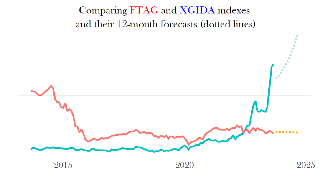
Based on the above plot, it appears that the primary index that moves the fund will maintain a relatively stable position for the next 12 months. So, I will consider it not a profitable investment.


Leave a comment